Data Primer: Percents Versus Counts

It’s pretty easy to assume that when looking at data, percents tell a better story than raw counts. Since the numbers are normalized, they can be easier to compare across geographies, and more clearly show the proportion of a total. If you know nothing about a city, it might not mean a lot to hear that, for example, 392,974 people in Washington, D.C. are non-White. But hearing that that’s 59.63% of the population might give you a better sense of the demographic makeup of the city.

In the map below, the percent of workers who are unemployed is clearly higher in West Virginia than in the Washington, D.C., metro area. This fits neatly with the narrative of high unemployment in the coal-mining regions of Appalachia.

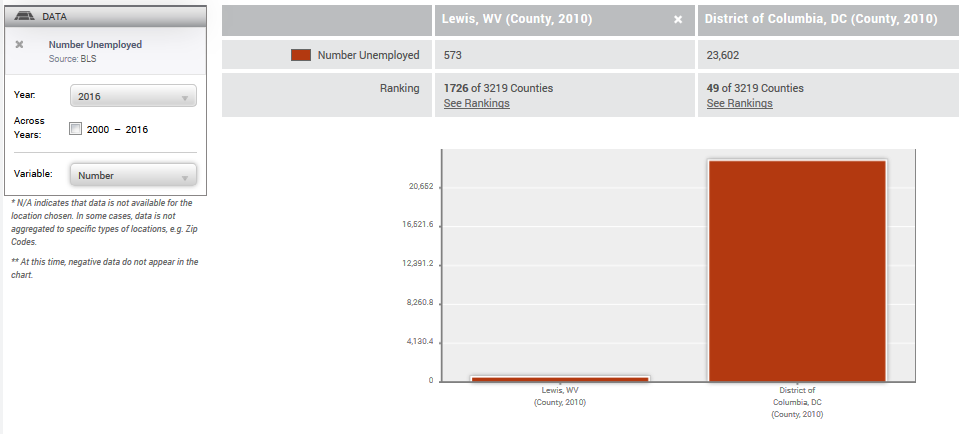
Looking at the same map, but with counts instead of percents, creates a completely different impression: now unemployment looks to be a bigger issue in Washington than in Lewis, West Virginia. But of course, there are a lot more people living in Washington than in Lewis.

So which is right? Is unemployment worse in Washington or West Virginia? That depends on what question you’re asking.

There are circumstances where counts are more useful than percents. Let’s say you want to open a job training facility in the mid-Atlantic. You aren’t necessarily interested in finding the place with the highest unemployment rates, because you’re more concerned with training as many workers as possible. Washington, D.C., might have a pretty low unemployment rate, but it has about 23,000 more unemployed workers than Lewis, W.V.: clearly, a much larger market for your training facility.

This sort of scenario isn’t the only time counts triumph over percents. Perhaps the most important reason in data analysis to use counts is to avoid falling into a percent trap, particularly a percent change trap.

Consider this: You’ve finally finished preparing a report on the economic outlook for Lewis, W.V., and you can’t believe how things have improved; in the 26452 zip code, mining jobs increased by 14% over the prior year! Is this really much of an improvement though? That 14% amounted to only ten new jobs.

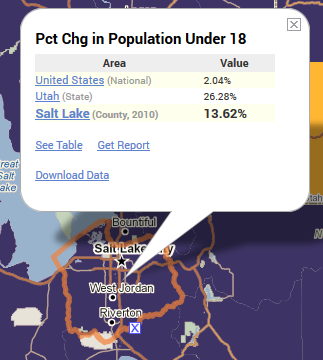
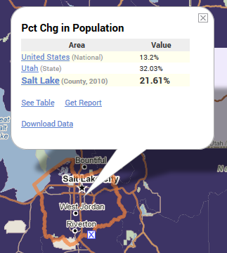
Another thing to watch out for with percent changes is that the change you see might reflect a change in the makeup of the area, or just a change in total population. Since 2000, the under 18 population in Salt Lake County, Utah, has grown by 13.62%. You might think there’s a surge of youth there. But the total population has grown 21.61%. The proportion of the population that’s under 18 has actually gone down relative to the rest of the growing population.

And when working with smaller numbers, particularly a small denominator, using percents tends to exaggerate the data, often to the point of misleading, or prompting inaccurate conclusions. For some datasets, such as those from the American Community Survey (ACS), we suppress percents where the denominator is less than 10, to avoid these misleading percents. (You can see whether there are suppressions by reading the data descriptions, which you can access by clicking on the label above the map.)

What does all this mean for the battle between percents and counts? Well, a percent is a standardized proportion—it demonstrates the relationship of a smaller segment to the whole. A count, on the other hand, is better at indicating the sheer size of something, or capturing small changes, regardless of other groups in the total population.

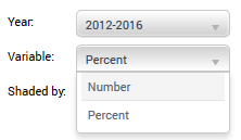Lots of indicators on PolicyMap have both numbers and percents available. Just go to the “Variables” menu in the map legend.

One rule of thumb you might use: If you want a sense of the character of a place, go with percent. If you want to know the size of a group and don’t care about people not part of that group, go with count. As always, though, use your judgement, since each use case is a little different.